Next: Correspondence Analysis
Up: Methods
Previous: Edge detection
Line Extraction
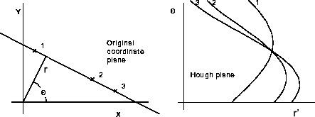
A line is defined as a set of points which are connected and form a straight line. It can be completely described through the start point and end point. There are different techniques for finding straight lines. The most popular one is the Hough transform. The basic idea of this technique is to find curves that can be parameterized, like lines, polynomials, circles, etc. in a suitable parameter space. The detection of straight lines in images will be shortly discussed because it is the main feature used in the proposed approach. Let us assume that the line is described in parameterized form
![]()
![]() , where
, where ![]() is the perpendicular distance from the origin and
is the perpendicular distance from the origin and ![]() the angle of the
the angle of the ![]() -coordinate with the normal. For any point
-coordinate with the normal. For any point
![]()
![]() on a straight line,
on a straight line, ![]() and
and ![]() are constant. Points in the cartesian image space maps to curves in the polar Hough parameter space. This point-to-curve transformation is called Hough transform. Points which are collinear in the image space intersects at a common point
are constant. Points in the cartesian image space maps to curves in the polar Hough parameter space. This point-to-curve transformation is called Hough transform. Points which are collinear in the image space intersects at a common point
![]()
![]() . Figure 3.8 shows how three lines are mapped into the parameter space. The transformation is implemented by quantizing the Hough parameter space into finite intervals, called accumulator cells. For every
. Figure 3.8 shows how three lines are mapped into the parameter space. The transformation is implemented by quantizing the Hough parameter space into finite intervals, called accumulator cells. For every ![]()
![]() , the parameters
, the parameters
![]()
![]() are computed and the accumulator at position
are computed and the accumulator at position
![]()
![]() is incremented. Peaks in the parameter space represent a straight line in the image space.
is incremented. Peaks in the parameter space represent a straight line in the image space.
 |
The main disadvantage is that it needs a lot of computational effort to transform the image into the hough-space and the output is a parametric description of a line, thus the starting and end point are not known and it needs some comparisons to find the starting and end point. Another way is to define a convolution mask which detects lines. The main disadvantage with this method is that every mask only finds lines that have a certain direction.
Another approach is to follow edge points iteratively and use the attitude of the found edge points as a reference to decide whether the following set of edge points seems to be in a line with the same attitude or not. The proposed work uses such a method.
A linear list is used to store the lines. A list element (line) consists of the following attributes
- Point start
- Stores the image coordinates of the point, where the line has its origin.
- Point end
- Stores the image coordinates of the point, where the line ends.
- Point cp
- The compare-point stores the image coordinates of the point, that is used to calculate the disparity between this line and the corresponding line in the other image. In other words, if

 is the line in the left image and
  its corresponding line in the right image, then the cp for is defined as
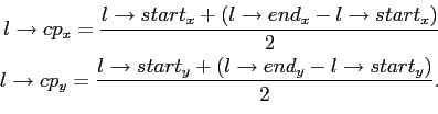

The cp for is defined as the point of intersection between a horizontal line
  , that has its origin in
  , and .
 - Real direction
- Stores the direction of the line, which is computed by adding up the directions of the edge pixels that are considered to lie on the line. The resulting direction is mainly used to find corresponding lines in other images, as well as finding corresponding object lines.
- Digit length
- Stores the length of the line. It is increased for every pixel that is added to the line.
- Digit counterX
- Counter of steps in x direction. It is increased or decreased in every iteration, dependently on the chosen direction.
- Digit counterY
- Counter of steps in y direction. It is increased or decreased in every iteration, dependently on the chosen direction.
- Digit disparity
- Disparity,

 if no disparity is found, or the disparity in pixels if a corresponding line has been found.
 - Real hitRateDisp
- Stores the rating of the correspondence between this line and a line in the other image. The line with the best rating is chosen, otherwise the rating is set to a value which is equivalent to .
- Real hitRateObj
- is the quality of the found object line or if no line is found.
- Real xw
- Stores the x-coordinate of the line in the world coordinate system.
- Real yw
- Stores the y-coordinate of the line in the world coordinate system.
- Real zw
- Stores the z-coordinate of the line in the world coordinate system.
- LineList* next
- Pointer to the next element of the line list or NULL at the end of the list.
- LineList* corrEdge
- Pointer to the corresponding line in the other image or NULL if no line is found.
- EdgeList* corrObj
- Pointer to a line that seems to belong to the other side of this line i.e. the two lines of a goal or a robot.
First of all everything is set to 0, except the disparity and both hit rates, which are all set to ![]()
![]() . A LIFO (last in, first out) list
. A LIFO (last in, first out) list ![]() of length
of length ![]() is created, which stores the chosen directions. The algorithm controls every pixel in the image whether it is an edge pixel. The search starts at the top-left of the image and searches from left to right and top to bottom. For vertical lines it is proven that when an edge pixel is found and it belongs to a line, the pixel is the first point of the line. This is not true for lines that are almost horizontal, but it can be ignored because horizontal lines cannot be used to calculate disparity and thus they are not searched for.
is created, which stores the chosen directions. The algorithm controls every pixel in the image whether it is an edge pixel. The search starts at the top-left of the image and searches from left to right and top to bottom. For vertical lines it is proven that when an edge pixel is found and it belongs to a line, the pixel is the first point of the line. This is not true for lines that are almost horizontal, but it can be ignored because horizontal lines cannot be used to calculate disparity and thus they are not searched for.
If an edge pixel is found and it is not already processed, the start and end points of the line list are set to its coordinate. Then the algorithm tries to follow the edge pixels, starting from the actual point, until the length of the line has reached a given threshold ![]()
![]() . During the process of following a line, pixels that seem to be more likely to lie on a straight line are preferred. This is necessary, otherwise the algorithm would always prefer a given direction.
. During the process of following a line, pixels that seem to be more likely to lie on a straight line are preferred. This is necessary, otherwise the algorithm would always prefer a given direction.
If a connection between a line point and one of its neighbour points, that can be used to continue the search, exists, the direction in which the new point can be found is stored. See Table 3.2 for possible directions and their encodings.
If no connection exists the algorithm stops and the pixels that are already in ![]()
![]() will be marked as processed. Then it continues searching edge pixels that are not processed yet. But if the length of the line reaches the threshold
will be marked as processed. Then it continues searching edge pixels that are not processed yet. But if the length of the line reaches the threshold ![]() , the attitude
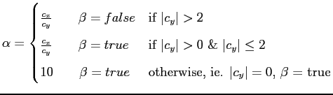
, the attitude ![]() of the first part of the line is computed.
of the first part of the line is computed. ![]() is now totally filled, that means if we add another direction, the oldest element will be shifted out of the list. Let us assume that
is now totally filled, that means if we add another direction, the oldest element will be shifted out of the list. Let us assume that ![]() is the counter in x direction,
is the counter in x direction, ![]() is the counter in y direction and
is the counter in y direction and ![]() is a boolean variable, then
is a boolean variable, then ![]() can be computed as
can be computed as
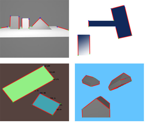
A linear list of lines is the result of this procedure. Figure 3.9 shows an image in which straight lines are searched.
 |
Unfortunately, edge pixels are not always connected. Thus, after the line list has been generated it tries to connect lines if they have approximately the same attitude, e.g. the absolute difference of two lines is below a threshold, and the end point of one line is near the start point of the other or vice versa.
Next: Correspondence Analysis
Up: Methods